A mathematical model of the coupling between segmental oscillators

The implementation of the Central Pattern Generator (CPG) Model is quite important in the development of locomotion control algorithms for robots. In this note, we will rewind the induction of a simple mathematical model for CPG.

Reference
The nature of the coupling between segmental oscillators of the lamprey spinal generator for locomotion: A mathematical model

Basics and Assumptions

The fundamental characteristics of the intact cord which any model must reproduce:

• There is a $\pi$ phase difference between left and right roots within individual segments: such intrasegmental locking is apparently stronger than intersegmental coupling.
• All segments are (to first order) frequency and phase locked, although variations and “hunting” about equilibrium can occur.
• There is a phase lag (constant to first order) from head to tail.

Thus we can make some assumptions based on these principle and experimental result.

Assumption1 oscillators
A neuronal oscillator, or pair of oscillators, is associated with each segment. We shall argue that simple phenomenological observations lead to a model which is adequate for our present purpose: that of studying the effects of intersegmental coupling.

Assumption2 coupling
Each segmental oscillato or pair of oscillators is coupled to its immediate neighbors and also possibly to distant oscillators. Each oscillator may also be connected to a central “control line” involving certain long axons in the medial tract.

Mathematical Model Induction

The individual Oscillator or Oscillator Pair

Observation
Any dynamical system modelling such a segmental oscillator should have an attracting limit cycle, $\gamma$.

Letting $\mathbf{x}=\mathbf{x}(t)=(x_1(t), x_2(t),…, x_n(t))$ be an n-vector of the relevant variables, a typical model might be an ordinary differential equation of the form

\[\dot{\mathbf{x}}=\mathbf{f(x)}\tag{2.1}\]

Since that the nature of the oscillator is still unknown, the model does not require detailed specification of the variables $\mathbf{x}$.

First important step
Choose a local coordinate system based on the periodic orbit $\gamma$, which forms a closed curve in the state space. (See more details in the original paper)

In terms of this parameterization, we have

\[\dot{\mathbf{r}}=\mathbf{f}_1(\mathbf{r},\theta)\tag{2.2}\] \[\dot{\theta}={\omega}+f_2(\mathbf{r},\theta)\tag{2.3}\]

where $\mathbf{f}_1(\mathbf{0},\theta)=\mathbf{0}$, $f_2(\mathbf{0},\theta)=0$ and $T=2\pi/\omega$ is the period of the oscillator. The function $\mathbf{f_1}$ and $f_2$ are necessarily of period $2\pi$ with respect to $\theta$.

We can assume that the system is structurally stable, then it follows that $\gamma$ is a hyperbolic attractor. Thus in studying steady solutions in the absence of external excitation, we need merely consider the single scalar phase equation. (This part needs further exploration, including grasping the theory fundamentals, and so on.)

\[\dot{\theta}=\omega\tag{2.4}\]

with solution

\[\theta(t)=\theta(0)+\omega t\tag{2.5}\]

The Chain of Oscillators

A typical member of N oscillators set being

\[\dot{\mathbf{x}_j}=\mathbf{f}_j(\mathbf{x}_j)+\mathbf{g}_j(\mathbf{x}_1,...,\mathbf{x}_N,\alpha)\tag{2.9}\]

where $\mathbf{g}$ is the coupling function, involving the dynamics of the other $N-1$ oscillators, and including a vector of coupling coefficients $\alpha$. $\mathbf{g_j}(\mathbf{x_1},…,\mathbf{x_N},0)=0$. Each oscillator exhibiting a stable limit cycle $\gamma _j$.

Assumption weak coupling
We assume that the coupling is relatively weak, so that $|\alpha|$ is small and $|\mathbf{g}|\ll|\mathbf{f}|$. In such case the limit cycles of the uncoupled oscillators are each slightly perturbed and one can continue touse the phase coordinates $\theta _j$, and amplitude $\mathbf{r}_j$ to characterize the state of each oscillator.

In this way one obtains sets of equations of the form

\[\begin{split} \dot{\mathbf{r}_j}&=\mathbf{f}_{j1}(\mathbf{r}_j,\theta _j)+\mathbf{g}_{j1}(\mathbf{r}_1,...,\mathbf{r}_N,\theta _1,...,\theta _N,\alpha) \\ \dot{\theta _j}&=\omega _j+{f}_{j2}(\mathbf{r}_j,\theta _j)+{g}_{j2}(\mathbf{r}_1,...,\mathbf{r}_N,\theta _1,...,\theta _N,\alpha) \\ \end{split}\tag{2.10}\]

Expanding this about $\mathbf{r_j}=0$ in Taylor series, one eventually obtains approximate phase equations for weakly coupled oscillators in the form

\[\dot{\theta _j}=\omega _j+{h_{j}}(\theta _1,...,\theta _N,\alpha)\tag{2.11}\]

from which all the amplitudes are absent.

We now ask what form might the functions $h_j$ be expected to take. Here we consider a linear coupling model. The system will obey

\[\dot{\mathbf{x}_i}=\mathbf{f}_i(\mathbf{x}_i)+\sum_{j=1}^{N}\mathbf{A}_{ij}\mathbf{x}_j\tag{2.12}\]

where $\mathbf{A}_{ij}$ are matrices of coupling coefficients multiplying the vectors $\mathbf{x}_j$.

In the case of weak coupling such a system leads to

\[\dot{\theta _i}=\omega _i+\sum_{j=1}^N{\alpha_{ij}}h(\theta_j-\theta_i)\tag{2.13}\]

where $h$ is a bounded periodic function of its argument.

The simplest periodic function $h(\phi)=\sin\phi$ arises in cases in which the unperturbed uncoupled limit cycles are sinusoidal.

Compared with PRC (pahse response curve), we arrive at

\[\dot{\theta _i}=\omega _i+\sum_{j=1}^N{\alpha_{ij}}\sin(\theta_j-\theta_i)\tag{2.14}\]

Here $\alpha_{ij}$ represents the strength of the coupling effect of the $j$th oscillator on the $i$th oscillator.

Analysis of the Mathematical Model

Nearest Neighbor Coupling

The simplest model is one in which each oscillator is coupled only to its nearest neighbors. Letting $\phi_{j}=\theta_j-\theta_{j+1}$ and $\Omega_j=\omega_j-\omega_{j+1}$, further assume that all upward coupling strengths $\alpha_{j,j+1}$ are equal to $\alpha_u$ and all downward strengths $\alpha_{j,-1}$ are equal to $\alpha_d$, we have

\[\dot{\Phi}=\mathbf{\Omega}+\mathbf{BS} \tag{3.3}\label{eq:3.3}\]

where

\[\Phi=\begin{bmatrix} \phi_1 \\ \vdots \\ \phi_{N-1} \\ \end{bmatrix} \ \ \ \ \mathbf{S}=\begin{bmatrix} \sin\phi_1 \\ \vdots \\ \sin\phi_{N-1} \\ \end{bmatrix} \ \ \ \ \mathbf{\Omega}=\begin{bmatrix} \Omega_1 \\ \vdots \\ \Omega_{N-1} \\ \end{bmatrix}\tag{3.4}\label{eq:3.4}\]

are $N-1$ vectors and

\[\mathbf{B}= \begin{bmatrix} -(\alpha_d+\alpha_u) & \alpha_u & & & \\ \alpha_d & -(\alpha_d+\alpha_u) & \alpha_u & \\ & & \cdots & \\ & & \alpha_d & -(\alpha_d+\alpha_u) \\ \end{bmatrix}\tag{3.5}\]

is a tri-diagonal $(N-1)\times(N-1)$ matrix. We shall be especially interested in $1:1$ phase locked solutions, in which all oscillators exhibit the same frequency. If any phase locked solutions exist, they are given by

\[\mathbf{S=-B^{-1}\Omega}\tag{3.6}\]

Example.1 3-oscillator system

\[\begin{bmatrix} \sin \phi_1 \\ \sin \phi_2 \\ \end{bmatrix} =\frac{1}{\alpha_d^2+\alpha_d\alpha_u+\alpha_u^2} \begin{bmatrix} \alpha_d+\alpha_u & \alpha_u \\ \alpha_d & \alpha_d+\alpha_u \\ \end{bmatrix} \begin{bmatrix} \Omega_1 \\ \Omega_2 \\ \end{bmatrix}\tag{3.9}\]

which reduces to

\[\sin\phi_1=(2\Omega_1+\Omega_2)/3\alpha \quad sin\phi_2=(\Omega_1+2\Omega_2)/3\alpha\tag{3.10}\]

if $\alpha_u=\alpha_d=\alpha$. Thus stable phase locking occurs if and only if

\[\max\{|2\Omega_1+\Omega_2|,|\Omega_1+2\Omega_2|\}\lt|3\alpha|\tag{3.11}\]

Computations for longer chains of oscillators rapidly become awkward. Here we may consider the constant indentical segemt to sgement phase lag case, i.e. $\theta_j-\theta_{j+1}=\phi_j=\delta$. We require

\[\begin{split} \Omega_1+[-(\alpha_d+\alpha_u)+\alpha_u]\Delta&=0 \\ &\ \ \vdots\\ \Omega_j+[\alpha_d-(\alpha_d+\alpha_u)+\alpha_u]\Delta&=0\\ &\ \ \vdots\\ \Omega_{N-1}+[\alpha_d-(\alpha_d+\alpha_u)]\Delta&=0\\ \end{split}\tag{3.12}\label{eq:3.12}\]

where $\Delta=\sin\delta \gt0$. This implies that $\Omega_j=0$ for $j=2,\ldots,N-2$ and $\Omega_1=\alpha_d\Delta$, $\Omega_{N-1}=\alpha_u\Delta$, or

\[\begin{split} \omega_j&=\omega\quad{\text{for all}}\quad j\neq 1,N\\ \omega_1&=\omega+\alpha_d\sin\delta\gt\omega\\ \omega_N&=\omega-\alpha_u\sin\delta\lt\omega \end{split}\tag{3.13}\]

To study the stability of this solution, we linearize $\eqref{eq:3.3}$ about the fixed point $\phi_j=\delta$ to obtain

\[\dot{\xi}=\mathbf{B^{'}}\xi\]

where $\mathbf{B^{‘}}=\mathbf{B}\cos\delta$, and $\delta$ is a small angle (Here we also assume $\sin\phi_j=\sin(\phi_j-\delta)\cos\delta=(\phi_j-\delta)\cos\delta$ when $\phi_j$ is near $\delta$). If, as is the case in our observations, $\delta$ is a small angle, so that $0\lt\cos\delta\lt1$, it can be shown that all eigenvalues of $\mathbf{B^{‘}}$ have negative real parts and thus that the uniform phase lagged solution is asymptotically stable.

Conclusion
If the nearest neighbor coupling predominates and the rostral oscillator runs appreciably faster, and the caudal oscillator appreciably slower than the central portion of the cord, then stable traveling wave solutions result.

An alternate approach to auusming a constant phase lag $\delta$ is to take each oscillator’s frequency $\omega_j$ to be smaller than its predecessor’s, i.e. $\omega_{j-1}$, by a fixed amount $\varepsilon$. i.e.

\[\omega_j-\omega_1-(j-1)\varepsilon,\quad j=2,\ldots,N\]

See more details in the paper, here we will find

\[\sin\phi_j=\frac{\varepsilon}{\alpha}\frac{j}{2}(N-j),\quad j=1,\ldots,N-1\tag{3.14}\]

Three and N Oscillators With Long Distance Coupling

Here we take three oscillators, with identical nearest neighbor coupling coefficients $\alpha$, and distant coupling $\beta$ between oscillators 1 and 3 as an example. The appropriate differential equations are

\[\begin{split} \dot{\theta_1}&=\omega_1+\alpha\sin(\theta_2-\theta_1)+\beta\sin(\theta_3-\theta_1)\\ \dot{\theta_2}&=\omega_2+\alpha\sin(\theta_1-\theta_2)+\beta\sin(\theta_3-\theta_2)\\ \dot{\theta_3}&=\omega_3+\alpha\sin(\theta_2-\theta_3)+\beta\sin(\theta_1-\theta_3)\\ \end{split}\tag{3.15}\label{eq:3.15}\]

We first note that if a phase locked solution exists, then $\dot{\theta_1}=\dot{\theta_2}=\dot{\theta_3}$ and the frequency ($\overline{\omega}$) of this solution is

\[\overline{\omega}=\frac{\omega_1+\omega_2+\omega_3}{3}\tag{3.16}\]

i.e. the symmetric coupling does not weight any particular oscillator. We next let $\phi_1=\theta_1-\theta_2$, $\phi_2=\theta_2-\theta_3$, and subtract the components of $\eqref{eq:3.15}$ pairwise to obtain

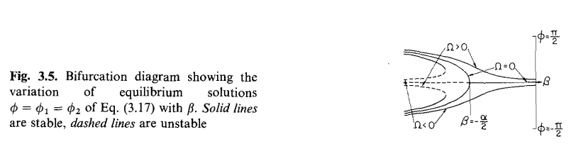
\[\begin{split} \dot{\phi_1}&=\Omega_1-2\alpha\sin\phi_1+\alpha\sin\phi_2-\beta\sin(\phi_1+\phi_2)\\ \dot{\phi_2}&=\Omega_2+\alpha\sin\phi_1-2\alpha\sin\phi_2-\beta\sin(\phi_1+\phi_2) \end{split}\tag{3.17}\label{eq:3.17}\]

To seek solutions we first set $\Omega_1=\Omega_2=0$ ($\omega_1=\omega_2=\omega_3$, indetical oscillators.) In this case $\eqref{eq:3.17}$ has either 4 or 6 fixed points. We assume that $\alpha\gt0$ (excitatory nearest neighbor coupling), but that $\beta$ can take either sign. Thus by setting $\phi_1=\phi_2=\phi$ we have

\[(2\beta\cos\phi+\alpha)\sin\phi=0\]

If $\beta\lt-\alpha / 2$, corresponding to relatively strong, inhibitory coupling between oscillator 1 and 3, then two stable solutons correspondng to phase lagged (forward) and phase leading (backward) traveling waves appear, with $\phi_j=\theta_j-\theta_{j+1}=\cos^{-1}(-\alpha/2\beta)$, while the in phase solution ($\phi_j=0$) becomes unstable. Uniform detuning $\Omega_1=\Omega_2=\Omega\ne0$ shifts these solutions as indicated in the bifuraction diagram of $\eqref{fig3.5}$.

\[\text{Bifuraction Diagram}\tag{fig3.5}\label{fig3.5}\]

Passing to the case of $N$ oscillators with only the first and last coupled at long distance, again with strength $\beta$, and the central ones coupled to the nearest neighbors alone, we obtain, for the case of identical oscillators ($\Omega_j=0$)

\[\begin{split} -2\alpha\sin\phi_1+\alpha\sin\phi_2-\beta\sin(\sum_{k=1}^{N-1}\phi_k)&=0\\ &\ \ \vdots\\ \alpha\sin\phi_{j-1}-2\alpha\sin\phi_j+\alpha\sin\phi_{j+1}&=0\\ &\ \ \vdots\\ \alpha\sin\phi_{N-2}-2\alpha\sin\phi_{N-1}-\beta\sin(\sum_{k=1}^{N-1}\phi_k)&=0 \end{split}\tag{3.19}\]

Thus we find that traveling wave solutions with phase lag $\phi_j=\overline\phi$, representing both forward and backward going waves, are possible for values of $\alpha$, $\beta$ for which

\[\beta\sin[(N-1)\overline\phi]+\alpha\sin\overline\phi=0\]

has nontrivial solutions.

In particular, from $\eqref{fig3.5}$, the model exhibits, for all $\Omega$, stable forward running phase locked solutions when the long distance coulpling is inhibitory and sufficiently strong for a given excitatory nearest neighbor coupling ($-\beta\gg\alpha\gt0$).

Conclusion
Chains of identical oscillators with nearest neighbor coupling plus irect rostral-caudal inhibitory coupling can also exhibit traveling waves of the type observed, although such stable waves appear in pairs, with both forward and backward going waves.

Problems
We remark that while lampreys are known to have the ability to swim backwards, in almost all cases of stable fictive swimming observed in our in vitro preparations forward traveling waves with the rostral part leading are observed. Frequently in the fictively swimming dogfish (Grillner, 1975) and occasionally in an isolated lamprey spinal cord, one of the central oscillators will take the lead, a phenomenon for which this model with long distance coupling cannot account (although the model with nearest neighbor coupling, $\eqref{eq:3.12}$, can exhibit this behavior).

Trainsients, Loss of Locking and Drifting with Weak Coupling

An alternative approach to considering the phase locked solutions of $N$ coupled oscillators is to consider the general (not necessarily phase locked) behavior of a smaller system of, say, two oscillators.

The differential equations describing a system of two oscillators are

\[\dot\theta_1=\omega_1+\alpha_u\sin(\theta_2-\theta_1)\tag{3.20}\label{eq:3.20}\] \[\dot\theta_2=\omega_2+\alpha_d\sin(\theta_1-\theta_2)\tag{3.21}\label{eq:3.21}\]

Thus we again obtain

\[\dot\phi=\Omega-k\sin\phi\tag{3.7}\]

where

\[\begin{split} \phi&=\theta_1-\theta_2=\text{phase difference}\\ \Omega&=\omega_1-\omega_2=\text{frequency difference}\\ k&=\alpha_u+\alpha_d=\text{net coupling}\\ \end{split}\]

If the net coupling $k$ is weak, $|k|\lt|\Omega|$, e.g. due to a lesion, then no phase locked solutions occur. Rather each of the two oscillators "drifts" in a manner which can be investigated by solving $\eqref{eq:3.20}$, $\eqref{eq:3.21}$ exactly.

See more discussions on “drifting” in the paper.

Discussion

Comparison of Experimental Lesion Results with Transient Model Behavior

The experimental and model systems clearly differ in several respects. For example, in both experiments illustrated the periods of the cord varied more chaotically in the experiment than in the model; furthermore, the simplified two oscillator model does not exhibit the $2 : 1$ and $3 : 1$ subharmonic locking which has been observed. In the two oscillator model discussed above, nearest neighbor coupling has been assumed and, as shown in section 3, the forward going traveling wave of normal fictive swimming results from that model if and only if the rostral oscillators run faster than the caudal oscillators. Since some cord fragments exhibit the opposite tendency, this model cannot encompass all the data. However, the 3-oscillator chain with ascending (long-distance) inhibitory coupling can exhibit forward going waves when either rostral or caudal oscillators are fastest. This is, of course, a generalization of the simple nearest-neighbor model and more complex, multi-oscillator generalizations may yield more realistic behavior.

Frequency Control

One factor which we have so far neglected in our model is frequency control. The decision to change swimming speed could be made in the brain with some of the tracts of the cord transmitting the signal which causes the release of the active compound. Some such control must exist, but the question remains as to the location of the fibers which control frequency, how they function and how they themselves are controlled.

Conclusions

In the models described above, several organizational schemes for the CPG are outlined. All have deficiencies at present but they permit some statements regarding central pattern generators in general. The first point of interest is that in all our models bidirectional coupling between the oscillators can generate a stable traveling wave. More striking is that in our simplest model, a single set of fibers is sufficient for the coordinating system to maintain proper phase coupling when the fish swims either forwards or backwards; it is necessary simply to retune the end oscillators (see section 3 above). Although the situation in the lamprey is more complex, this elegant mechanism could well apply in simpler 2 oscillator systems. One need not posit any complicated arrangement for reversing the direction of propagation; some control center could easily retune the oscillators when necessary. Whether other systems of multiple coupled oscillators such as that of the leech (Friesen and Stent, 1977) utilize this type of control mechanism is unknown, but could be tested.

It remains unclear how the lamprey cord is structured. First, more data are required to characterize more fully the function and anatomy of the cord. Second, we plan to add elements to the model which would control the frequency and to test other forms of coupling either separately or in combination with the present types. It is not possible to prove that a model is “correct”, but with such models as ours it should be possible to test assumptions and formulations which in turn should suggest further experiments and refinements of our concepts.